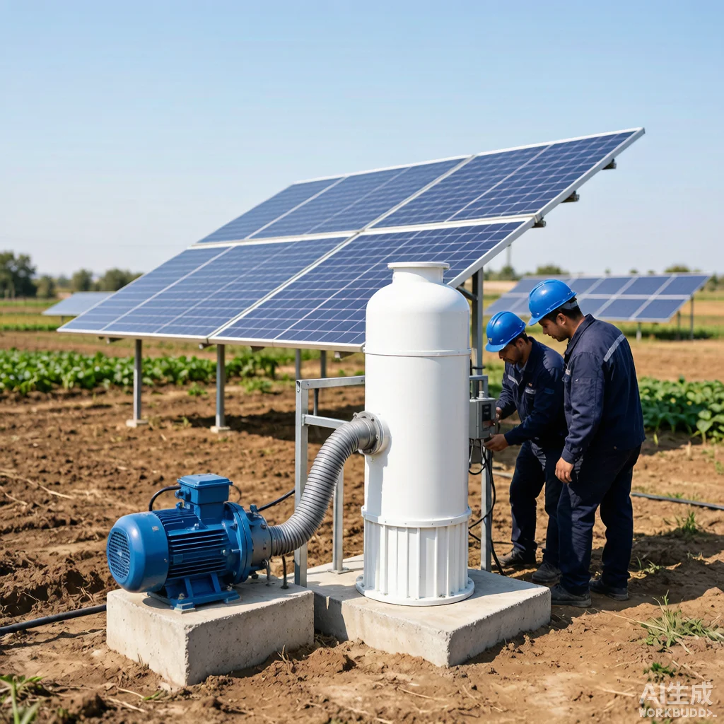
Advanced Solar Pump Performance Curve Interpretation Guide
Introduction
Pump performance curves are the primary engineering tool for selecting and sizing solar water pumping systems, yet their effective interpretation requires understanding not just the basic Q-H relationship but also efficiency characteristics, net positive suction head (NPSH) requirements, and the interaction between the pump curve and the available solar power curve. A common procurement error is to select a pump based solely on its rated duty point — the single flow-head combination where the manufacturer guarantees a specific efficiency — without analyzing whether the pump can operate efficiently across the range of conditions produced by variable solar irradiance throughout the day and across seasons. KINBO provides comprehensive performance curve documentation for all its pump models, including multi-speed curves, efficiency contour maps (efficiency islands), and NPSH curves, enabling system designers to make data-driven selection decisions that maximize daily water output and minimize energy waste. This article provides an advanced treatment of pump curve interpretation specifically for solar pumping applications, covering Q-H curve analysis, Best Efficiency Point (BEP) identification, NPSH margin determination for cavitation prevention, and the integration of pump performance data with solar array sizing calculations. The content is designed for engineers and technically proficient procurement professionals who need to move beyond basic pump selection and into optimized system design.
Table of Contents
Understanding Q-H Curves for Solar Applications
The Q-H curve (flow rate versus head) is the fundamental pump characteristic that defines the relationship between the flow a pump can deliver and the total dynamic head against which it must operate. For a centrifugal or mixed-flow pump, the Q-H curve is typically downward-sloping: as the discharge head increases (deeper water level, higher discharge point, or greater friction losses), the achievable flow rate decreases. The shape and slope of this curve have profound implications for solar pump performance under variable power conditions.
A steep Q-H curve — where flow changes relatively little over a wide range of head — is characteristic of high-head, low-specific-speed pump designs with narrow impeller passages and relatively large impeller diameters. These pumps maintain reasonably consistent flow as water levels fluctuate seasonally, but they are sensitive to head estimation errors: a 10% underestimation of TDH can result in a 20-30% overestimation of available flow if the operating point shifts significantly along a steep curve. Conversely, a flat Q-H curve — where flow changes dramatically with small head variations — is typical of low-head, high-specific-speed designs. These pumps deliver high flow at low head but experience rapid flow reduction if head increases beyond the design point. For solar applications where available power varies continuously, pump curve slope directly affects the daily flow variability: steep-curve pumps produce more consistent daily flow but require more precise head estimation, while flat-curve pumps are more forgiving of estimation errors but produce greater flow variability with changing irradiance.
For variable speed operation, the pump manufacturer typically provides a set of Q-H curves at different operating speeds (often shown at 10% or 20% speed increments), or alternatively provides the curve at rated speed with affinity law formulas to calculate performance at other speeds. The affinity relationships are: Q₂/Q₁ = N₂/N₁ (flow proportional to speed), H₂/H₁ = (N₂/N₁)² (head proportional to speed squared), and P₂/P₁ = (N₂/N₁)³ (power proportional to speed cubed). These relationships hold with reasonable accuracy for speed reductions down to approximately 50% of rated speed; below 50%, hydraulic efficiency degradation becomes significant and the cubic power relationship overestimates actual power savings. When interpreting multi-speed curves for solar applications, the key engineering task is to verify that the pump’s operating envelope — the range of flow-head combinations achievable across the expected speed range — encompasses the full range of site conditions (seasonal water level variation, varying discharge pressure requirements) with acceptable efficiency.
Efficiency Islands and Best Efficiency Point
The efficiency of a centrifugal pump varies across its operating range, reaching a maximum at the Best Efficiency Point (BEP) and declining as the operating point moves away from BEP in either direction — toward lower flow (left of BEP) or higher flow (right of BEP). Pump manufacturers represent this efficiency variation through efficiency contour lines, often called “efficiency islands,” superimposed on the Q-H curve. Each contour line connects operating points that achieve the same hydraulic efficiency, with the innermost contour representing the highest efficiency region surrounding the BEP.
For solar pump selection, the goal is not simply to match the rated duty point to the BEP, but to ensure that the pump’s BEP region encompasses the range of flow-head combinations the pump will traverse during a typical solar day. A pump whose rated duty point is exactly at BEP for the design head but whose efficiency drops below 60% at the reduced flow rates experienced during morning and afternoon low-irradiance hours will average 5-10 percentage points lower daily efficiency than a pump with a broader efficiency plateau that maintains above 70% efficiency across the full operating range. The width of the high-efficiency region is a function of pump hydraulic design: pumps designed with 3D-curved impeller vanes (as opposed to simpler 2D cylindrical vanes) and optimized volute or diffuser geometries typically achieve wider efficiency plateaus, often maintaining efficiency within 5 percentage points of BEP over a flow range of 70-120% of BEP flow.
The selection methodology for solar applications should therefore prioritize pumps whose efficiency at the estimated operating point plus-minus 20% flow variation remains above the manufacturer’s recommended minimum efficiency threshold. KINBO publishes efficiency island data for all pump models in its technical documentation, and its application engineering team can provide efficiency-versus-flow plots calculated at actual site head and speed conditions. For procurement specifications, requesting efficiency guarantees at three points — the rated duty point, 80% of rated flow, and 120% of rated flow — provides a more robust basis for comparing competing pump offerings than a single BEP efficiency number, which can be misleading when the pump operates away from BEP for significant portions of the day.
NPSH Curves and Cavitation Prevention
Net Positive Suction Head (NPSH) analysis is one of the most frequently overlooked aspects of solar pump selection, yet cavitation damage from inadequate NPSH margin is one of the most common causes of premature pump failure. NPSH has two components: NPSH Available (NPSHa), which is a function of the installation — atmospheric pressure, static water level, suction pipe friction losses, and vapor pressure of the water — and NPSH Required (NPSHr), which is a characteristic of the pump determined by its hydraulic design and operating point. Cavitation occurs when NPSHa falls below NPSHr, causing vapor bubbles to form on the low-pressure side of the impeller vanes and subsequently collapse violently as they enter higher-pressure regions, generating localized shock waves that erode impeller material.
The NPSHr curve provided by the pump manufacturer shows how NPSHr varies with flow rate. NPSHr typically increases with flow because higher flow velocities through the impeller eye create lower static pressures at the vane leading edges. For submersible pumps installed in boreholes, NPSHa is generally favorable because the pump is submerged, providing a positive suction head equal to the submergence depth plus atmospheric pressure head minus friction losses and vapor pressure. However, NPSHa can become marginal when the pump is installed at the minimum recommended submergence (just below the lowest expected pumping water level), when water temperature is elevated (water at 60°C has a vapor pressure of approximately 2 meters head versus 0.24 meters at 20°C), or at high-altitude sites where reduced atmospheric pressure lowers NPSHa by approximately 0.12 meters per 100 meters of elevation above sea level.
Industry standards recommend a minimum NPSH margin (NPSHa minus NPSHr) of 0.5-1.0 meters for most applications, with a 1.5-meter margin recommended for pumps operating at flows above 110% of BEP where cavitation risk increases. For solar pump installations at altitudes above 2,000 meters (common in Andean, East African highland, and Central Asian mountain sites), the NPSH calculation must explicitly account for the reduced atmospheric pressure, which at 3,000 meters elevation is approximately 70% of sea-level pressure, reducing NPSHa by approximately 3 meters compared to a sea-level installation with the same submergence. Where NPSH margin is found to be inadequate, solutions include specifying a pump with lower NPSHr (achieved through larger impeller eye diameter or inducer stage), installing the pump at greater submergence depth, or reducing the maximum operating speed (which shifts the NPSHr curve downward).
Using Curves for Solar Array Sizing
The integration of pump performance curve data with solar PV array sizing represents the final and most application-specific stage of pump selection. Unlike grid-powered pump applications where the motor can draw whatever power it requires up to the rated limit, a solar pump’s available power varies continuously with irradiance, and the pump must be able to operate efficiently across this variable power envelope. The array sizing methodology starts with the pump’s power-versus-flow curve — typically provided by the manufacturer or derived from the Q-H and efficiency curves using the relationship P_hydraulic (kW) = (Q × H × ρ × g) / (3.6 × 10⁶ × η), where Q is in m³/h, H in meters, ρ is water density (1,000 kg/m³), g is gravitational acceleration (9.81 m/s²), and η is pump efficiency at the operating point.
The critical parameter for array sizing is the pump’s power requirement at the design duty point, which determines the minimum PV array capacity needed to achieve the target daily water volume. However, sizing the array to exactly match the design-point power requirement is generally inadequate because: (a) PV panels rarely produce their rated STC (Standard Test Conditions) power in the field, achieving 80-90% of rated output under typical operating conditions (NOCT — Normal Operating Cell Temperature); (b) irradiance varies through the day, and pumping during the 2-3 hours around solar noon accounts for only 40-50% of total daily water production; and (c) the pump motor and controller have combined electrical efficiency losses of 10-20%. The recommended approach is to apply a derating factor of 0.75-0.85 to the STC panel rating to reflect realistic field conditions, and then size the array so that the derated power output at peak irradiance equals or exceeds the pump’s design-point power requirement by a margin of 10-15% to account for soiling, aging, and temperature-related efficiency losses.
For variable speed solar pump systems, an advanced sizing technique is to model the pump’s daily water output by integrating the instantaneous flow rate over the daily solar irradiance profile. This requires: (1) the pump’s Q-H curves at multiple speeds; (2) the site-specific TDH (accounting for drawdown variation with flow rate); (3) the pump’s power-versus-flow characteristics; (4) the solar array’s I-V curve and the MPPT controller’s operating characteristics; and (5) hourly or sub-hourly solar irradiance data (from TMY — Typical Meteorological Year — datasets, or satellite-derived irradiance data such as NASA POWER or Solargis). KINBO provides solar pump sizing software that automates this integration, accepting site coordinates for automatic irradiance data retrieval, well test data for TDH calculation, and pump model selection to generate daily, monthly, and annual water production estimates with associated confidence intervals. For procurement professionals evaluating competing proposals, requesting this level of sizing detail distinguishes suppliers with genuine application engineering capability from those offering generic, unvalidated performance claims.
Frequently Asked Questions
Q: How do you read and interpret a multi-speed pump performance curve for solar applications?
A: A multi-speed pump curve displays multiple Q-H curves, each corresponding to a different operating speed (typically expressed as a percentage of rated speed or as a specific RPM). The curve family is bounded by the maximum speed curve (100% rated speed, determined by the motor’s maximum frequency and the mechanical limits of the rotating assembly) and a practical minimum speed curve (typically 50-60% of rated speed, below which hydraulic efficiency degrades significantly and the affinity laws lose accuracy). For solar application analysis, the key steps are: (1) Plot the system curve — the relationship between head and flow for the specific installation — which is typically a parabolic curve starting at the static head and rising with the square of flow due to friction losses. (2) Identify the intersection points of the system curve with each speed curve; these are the operating points at that speed. (3) Verify that the required flow at the design head intersects the family of speed curves within the recommended operating range (typically 70-120% of BEP flow at each speed). (4) Check that the operating points at minimum speed (corresponding to early morning/late afternoon irradiance) remain above the minimum continuous flow specified by the manufacturer — typically 10-15% of rated flow for submersible pumps, below which inadequate motor cooling through water flow can cause overheating. (5) Confirm that the power requirement at each operating point, derived from the power curve or calculated from Q, H, and efficiency, is achievable from the PV array at the corresponding irradiance level.
Q: What are the consequences of operating a solar pump to the left of its Best Efficiency Point (BEP)?
A: Operating to the left of BEP (at lower-than-design flow rates) produces several detrimental effects that compound over time. Hydraulically, flow recirculation occurs within the impeller passages as the flow detaches from the vane suction surfaces, creating unstable flow patterns that generate pressure pulsations at frequencies typically 0.5-1.5 times the running speed. These pulsations transmit vibration to the entire pump assembly, accelerating bearing wear and potentially causing fatigue cracking of impeller vanes in pumps with high specific speeds. Mechanically, the radial thrust on the impeller increases as flow departs from BEP, particularly in single-volute pump designs where the pressure distribution around the impeller periphery becomes increasingly non-uniform. The resulting radial load on the shaft and bearings is approximately 2-3 times higher at 50% of BEP flow compared to operation at BEP. Thermally, reduced flow through a submersible motor reduces convective cooling, potentially causing the motor winding temperature to exceed the insulation class rating if the condition persists for extended periods — a particular concern for solar pumps during extended periods of low irradiance. For these reasons, industry guidelines recommend that pumps not be operated continuously at less than 40-50% of BEP flow. For solar applications where variable speed operation inherently shifts the operating point across a wide flow range, selecting a pump whose high-efficiency plateau extends sufficiently far to the left of BEP is critical to avoiding these long-term reliability issues. KINBO specifies the recommended continuous operating range (both minimum and maximum flow relative to BEP) in its pump technical datasheets.
Q: How does variable solar irradiance affect the pump performance curve and system operating point?
A: Variable solar irradiance does not change the pump’s Q-H curve itself (which is purely a function of pump geometry, speed, and fluid properties), but it changes the available electrical power, which in turn determines the pump’s achievable speed and consequently shifts the operating point along the system curve. As irradiance decreases during cloud passage or afternoon decline, the PV array’s power output drops, causing the controller’s MPPT algorithm to reduce the DC bus voltage and the VFD to correspondingly reduce the output frequency and voltage. The pump speed decreases, and the operating point slides down the system curve to a lower head and flow combination. The trajectory of the operating point during this transition is not arbitrary — it follows the intersection of the system curve with the successively lower speed curves. The critical engineering implication is that the pump’s efficiency at each of these transient operating points must remain acceptable, or the system wastes a disproportionate amount of the limited available energy during low-irradiance periods. This is why the efficiency plateau width is as important as the peak BEP efficiency for solar applications. A pump with 78% peak efficiency but a narrow efficiency range may average only 62% daily efficiency under variable irradiance, while a pump with 75% peak efficiency but a broad plateau may average 70% daily efficiency, ultimately delivering more daily water output. The system designer must also account for irradiance transients in the controller’s MPPT response time: a fast-moving cloud can cause irradiance to drop by 50-80% within seconds, and the controller must track this change without causing the pump to lose prime or enter an unstable oscillation. MPPT tracking speed is typically specified as a sweep frequency (how often the controller searches for the maximum power point, typically 5-20 Hz) and is an important controller specification to review alongside pump curve data.
Need expert assistance with solar pump performance curve analysis and system sizing? Contact KINBO for technical datasheets, sizing software, and application engineering support.
Related Articles
- Solar Pump Curves: Flow, Head, and Power Relationship Explained
- How to Calculate Total Dynamic Head for Solar Pump Selection